An ICLR 2026 Oral paper explainer: MoE needs a more aggressive data scaling strategy.
1. The short version
The central question of this work is simple:
Can we train an MoE LLM that matches a Dense LLM under the same total parameter count and the same training compute, so that the inference-time FLOPs reduction becomes an effectively free gain with respect to model size and training compute?
Our answer is:
- Under fixed total parameters and fixed training compute, if MoE wants to match Dense, the core cost is not parameters but tokens: it pays roughly times more consumed training tokens, where is the activation rate, i.e., activated parameters over total parameters. In exchange, MoE reduces per-token FLOPs to roughly of Dense.
- This bargain only works in a good activation-rate region. MoE is not “the sparser, the better”; across these experiments, the useful band is moderate, roughly 10%-30%, while larger model scales may expand or shift this region toward sparser MoEs.
- When unique data is limited, moderate data reuse can preserve much of the MoE advantage.
This answer is backed by a large experimental sweep, not a single cherry-picked run:
In other words, the practical recipe is:
Optimized MoE backbone + a suitable activation rate + aggressive token scaling, with moderate data reuse when unique tokens are limited.
2. Motivation: the blind spot---parameter subsidy
Two common comparison styles appear in the literature:
- Fix the data and training setup, then emphasize active-compute efficiency. DeepSeekMoE 16B is a typical example: trained on the same 2T-token corpus, it reports comparable performance to DeepSeek 7B Dense with only about 40% of the computation, and comparable performance to LLaMA2 7B, while using a larger total-parameter MoE reservoir [1].
- Fix the active expert budget or target per-token compute, then increase the number of total experts. Kimi K2’s sparsity scaling ablation is a clear example of this perspective [3].
Both perspectives are useful, but neither controls total parameters, which determine capacity, HBM footprint, checkpoint size, and the minimum deployment unit; in practice, when the batch size is large, almost all experts are activated somewhere in the batch. The sharper question is therefore: if Dense and MoE have the same total parameter count and the same training compute, can MoE still match or surpass Dense? A yes would mean the gain is not merely a parameter subsidy, but evidence that sparsity can become a real architectural advantage when trained correctly.
3. The resource equation
For a Dense model, the paper approximates per-token forward computation as:
Here denotes per-token forward FLOPs, denotes total non-embedding parameters, and absorbs Dense shape factors such as sequence length, model width, and FFN expansion ratio.
For an MoE model with the same total parameter count:
Here denotes activated parameters, is the activation rate, and absorbs the corresponding MoE shape factors. Once the backbone shape is fixed, and are approximately constant. The full parameterization from the paper is unpacked in English Appendix A, and the full notation table is in English Appendix D.
If denotes consumed training tokens and denotes total training compute, then equal training compute gives:
Rearranging gives:
This is the key trade-off.
At the same total parameter count, a 20% activation-rate MoE has roughly one fifth of the Dense per-token FFN-style compute, but to spend the same training compute it must process roughly 5x as many tokens, up to shape-factor corrections.
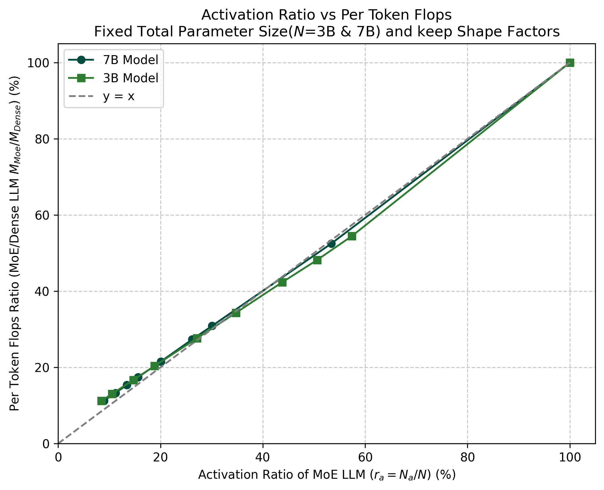
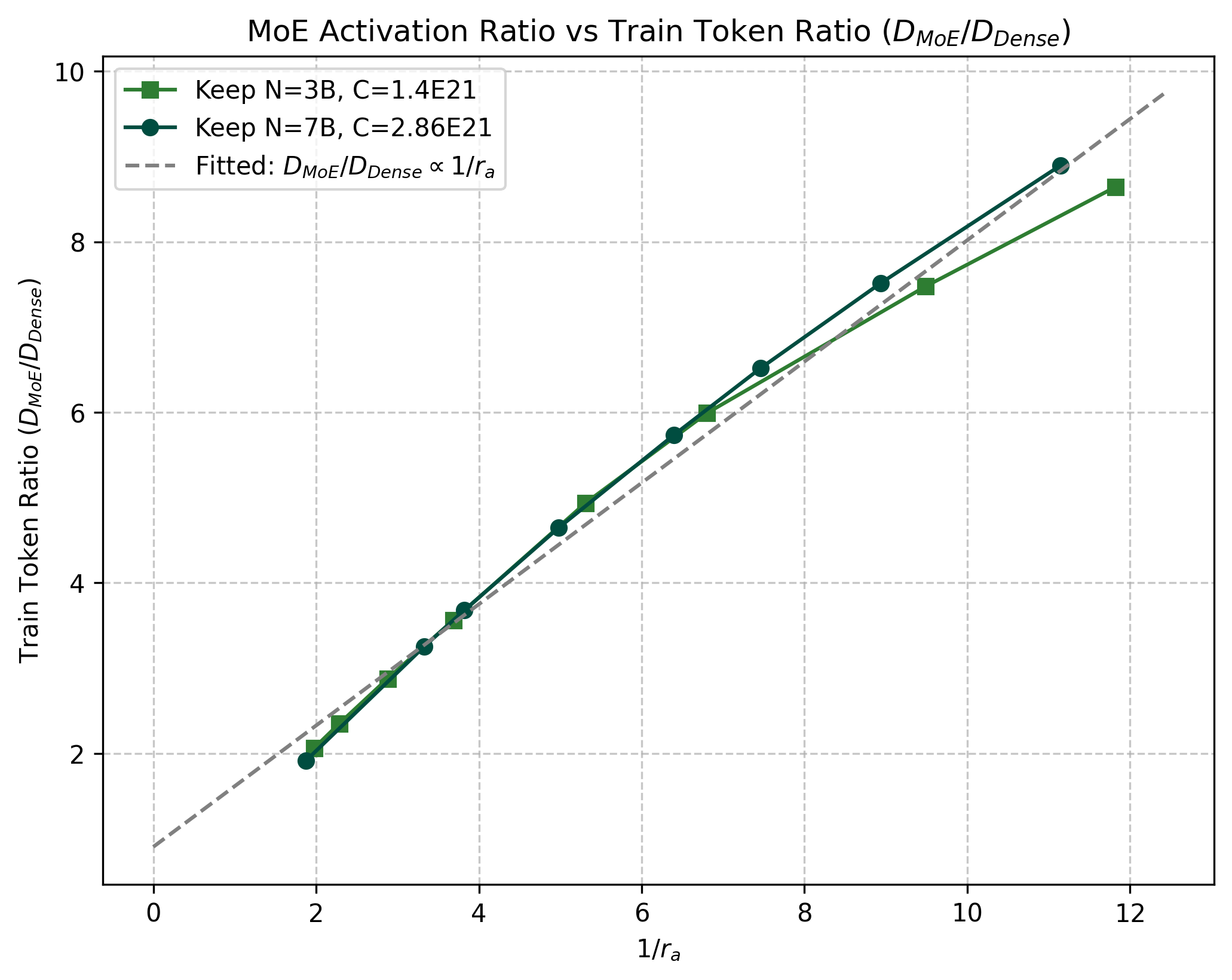
The paper also empirically verifies both sides of this relationship: MoE per-token FLOPs are close to linear in across the 3B and 7B settings (Figure 1a), and under equal compute, the consumed-token multiplier is close to linear in (Figure 1b).
4. The three-step methodology
Eqs. (2)-(3) imply that, after dropping the common forward/backward multiplier, MoE training compute behaves roughly as . A full compute-optimal MoE study would therefore have to sweep at least architecture, sparsity, total parameters , and the training-token ratio . This is much higher-dimensional than the usual Dense scaling-law sweep over and . Under a finite experiment budget, the paper chooses a greedy route instead: reduce the number of model configurations, but train each configuration deeply enough that the comparison is in a sufficiently trained regime, closer to how production SOTA models are trained.

Figure 2. Blog-native view of the paper’s three-step methodology: first optimize and lock the MoE backbone, then search activation rate under fixed N and C, and finally use data reuse to make the comparison strict under finite unique data.
The paper therefore adopts a greedy strategy: first give MoE a strong optimized backbone, then sweep under fixed total parameters N and training compute C, and finally test the effect of data reuse. The Dense baseline is also not arbitrary; it uses the optimal FFN ratio strategy, so the intended comparison is between a well-tuned Dense model and a well-tuned MoE family.
5. Step 1: Optimize the MoE architecture
MoE has more structural degrees of freedom than Dense. A Dense model is largely determined by its aspect ratio and FFN ratio. An MoE model also has to choose the Dense/MoE layer mix, whether to use shared experts, the routing top-K, routed and shared expert sizes, total expert count, and global shape ratios.
If these are not controlled, an activation-rate sweep can become meaningless. A bad result might simply mean the MoE backbone was bad. The architecture search narrows this design space into the backbone choices used for the later sweeps.
Table 1. Step 1 architecture-search conclusion table.
| Component | Conclusion used for the backbone |
|---|---|
| Layer arrangement | Use 1dense+SE: one initial Dense layer, followed by MoE layers with shared experts. |
| Gate normalization | Normalization reduces balance loss in the small-model ablations. |
| Top-K routing | Avoid both K = 1 and overly large K; use intermediate top-K choices whenever possible. |
| Shape ratios | The search supports a reasonable range rather than a single universal value: zeta around 60-120 is reasonable, and mu around 20 is reasonable. |
Step 1 is mainly about fairness. Before comparing MoE with Dense, the paper first gives MoE a strong backbone. After that, the activation-rate sweep asks a cleaner question: among well-constructed MoE models with the same total-parameter budget, which activation rate actually works best? Stabilizing kappa_MoE also helps the resource-equation analysis, but that is a secondary benefit. The detailed Step 1 experiments are in Appendix C.
6. Step 2: Search the optimal activation rate
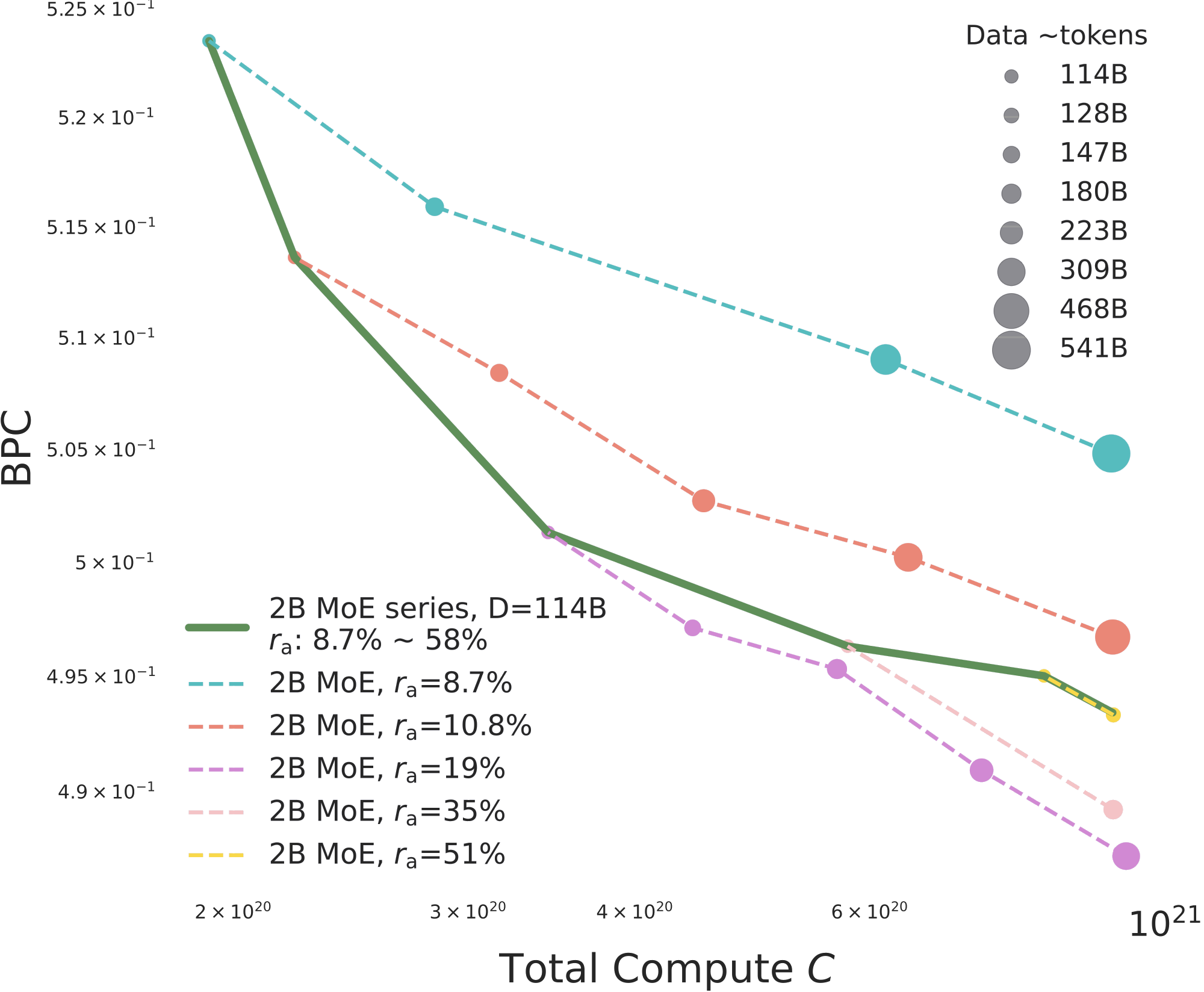
How to read Figure 3a. The x-axis is total training compute, and the y-axis is BPC, where lower is better. The bubble size encodes consumed training tokens. Each dashed line holds the activation rate fixed and increases tokens; along these lines, more tokens reduce BPC steadily, almost in a log-log linear pattern, which matches the usual data-scaling intuition. The solid green line instead holds the data budget at D = 114B and changes from sparse to dense. This separates two ways of spending more compute: feed more tokens at fixed , or activate more parameters at fixed data.
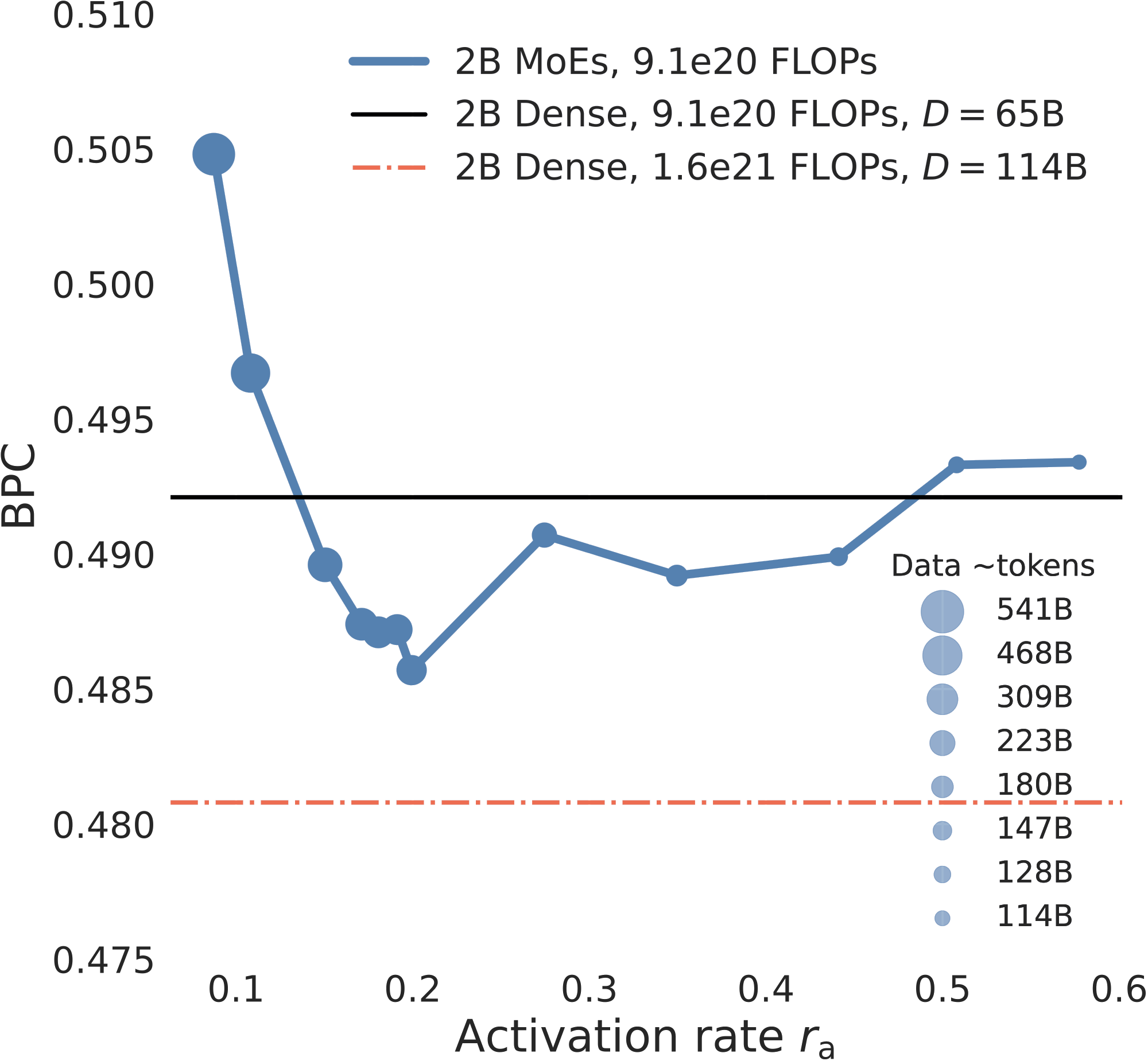
How to read Figure 3b. The x-axis is , and the y-axis is BPC. The blue curve is the 2B MoE family under the same total training compute. The bubble size again shows how many tokens each MoE consumes under that fixed-compute budget. The black horizontal line is the same-compute 2B Dense baseline, and the red dash-dot line is the stronger Dense baseline trained with more compute and more data.
Findings.
- At fixed , BPC follows the expected data-scaling trend as tokens increase. But when training tokens and total parameters are fixed, and training compute increases only because the MoE activates more parameters, the BPC-compute relationship is no longer the same smooth scaling curve. This is the first signal that an optimal activation region can exist.
- Under fixed total parameters and fixed compute, MoE is not “the sparser, the better.” The useful region is a moderate activation band, roughly 10%-30%, with the clearest 2B point near .
7. Step 3: Data reuse, 7B validation, and downstream value
7.1 Step3A: 3B activation-rate search under data reuse
The 3B experiment is the first stress test for data reuse. It keeps total parameters and training compute roughly fixed, then compares two MoE families: one with unique tokens close to the Dense-1C data budget, and one with a larger unique-token budget. The y-axis is Delta BPC against the Dense-1C baseline, so lower is better; negative values mean the MoE beats Dense-1C.
Figure 4 and Table 2 should be read together. The figure shows the full 3B activation-rate pattern, while the table focuses on the stricter MoE-65B setting: the cleaner test of whether MoE can stay competitive while using nearly the same amount of unique data as Dense-1C.
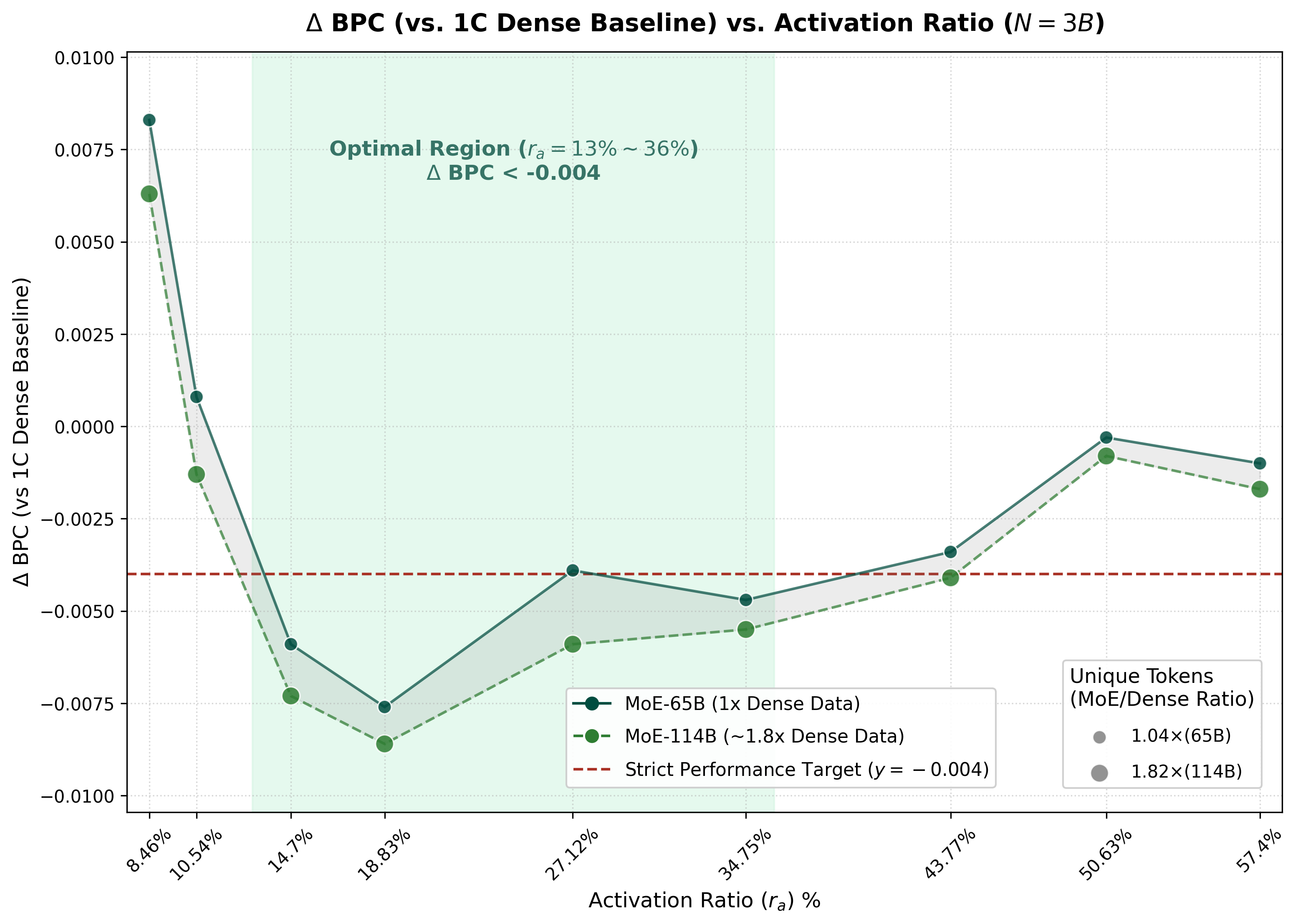
MoE-65B, where unique tokens are kept near the Dense-1C budget (1.04x, about 65B tokens). The dashed green line is MoE-114B, a looser setting with about 1.82x Dense-1C unique tokens. The red dashed line is the strict target Delta BPC = -0.004, and the shaded band marks the annotated optimal region.Table 2. 3B Step3A resource table. The selected MoE rows use nearly the same unique-token budget as Dense-1C, but consume more training tokens through reuse. BPC deltas are relative to Dense-1C, and lower is better.
| Model | C | ra | FLOPs/tok. | Train tok. | Unique tok. | Reuse | ΔBPC |
|---|---|---|---|---|---|---|---|
| Dense-1C baseline | 1.00x | 100.0% | 100.0% | 1.00x | 1.00x | 1.00 | 0.0000 |
| MoE-65B-Exp3 | 1.00x | 14.70% | 16.7% | 5.99x | 1.04x | 5.77 | -0.0059 |
| MoE-65B-Exp4 | 1.01x | 18.83% | 20.4% | 4.94x | 1.04x | 4.75 | -0.0076 |
| MoE-65B-Exp5 | 0.99x | 27.12% | 27.6% | 3.56x | 1.04x | 3.43 | -0.0039 |
| MoE-65B-Exp6 | 0.99x | 34.75% | 34.3% | 2.88x | 1.04x | 2.77 | -0.0047 |
The important reading is not that every reuse setting is equally good. It is that, even when unique tokens are almost fixed to the Dense-1C budget, a moderate activation rate can make MoE outperform Dense-1C under roughly equal total parameters and compute. The best row here is MoE-65B-Exp4 at , with Delta BPC = -0.0076.
7.2 Step3B: 7B data reuse, the sweet spot, and the resource table
At 7B, the paper switches to a harder baseline. Since the MoE models already surpass Dense-1C under equal total parameters and compute, Figure 5a uses Dense-2C as the reference line. The y-axis is Delta BPC against Dense-2C; below zero means the MoE is better than a Dense model trained with roughly twice the compute and twice the unique tokens.
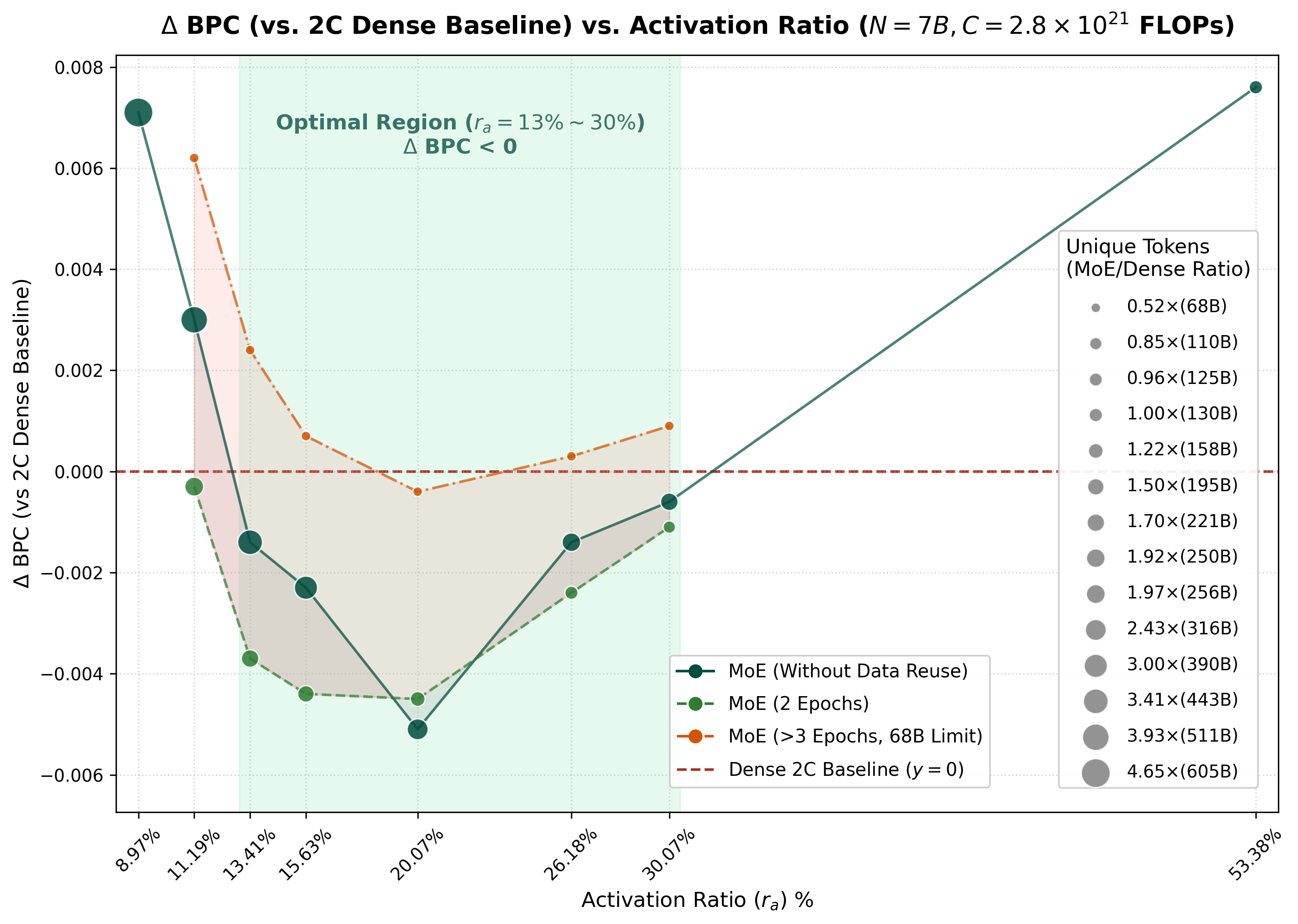
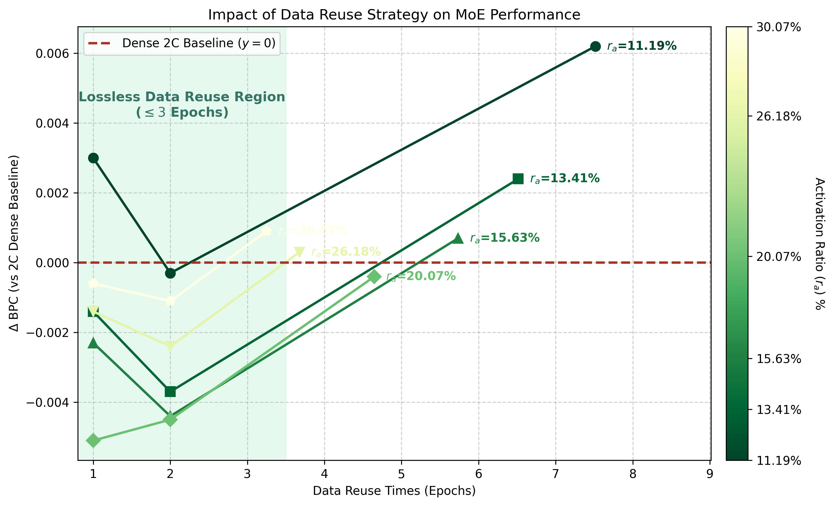
Together, Figures 5a and 5b show the same 7B trade-off from two angles. In Figure 5a, MoE without reuse can beat Dense-2C across a broad midrange but needs many more unique tokens; with two epochs, the same midrange still beats Dense-2C while using much less unique data; under the strict 68B cap, most activation rates fall short, but still matches Dense-2C. Figure 5b then makes the reuse axis explicit: moderate reuse can preserve or improve MoE performance, while excessive reuse degrades sharply, especially when the activation rate is too sparse.
Table 3. 7B Step3B resource table corresponding to Figures 5a and 5b. Deltas are relative to Dense-2C; lower BPC is better. The row to notice is MoE-68B at : same total-parameter scale, 68B unique tokens, 4.65 reuse epochs, only 21.5% per-token FLOPs, and BPC 0.4590, comparable to Dense-2C at 0.4594. This means that, with the right activation rate, MoE can still trade more consumed tokens for activation-rate-level per-token FLOPs even when unique tokens are tightly capped.
| Model / strategy | Unique tokens | Reuse epochs | FLOPs/token vs Dense | BPC | Delta BPC vs Dense-2C | |
|---|---|---|---|---|---|---|
| Dense-1C | 100.00% | 68B | 1.00 | 100.0% | 0.4736 | +0.0142 |
| Dense-2C | 100.00% | 130B | 1.00 | 100.0% | 0.4594 | 0.0000 |
| MoE-Unique | 11.19% | 511B | 1.00 | 13.3% | 0.4624 | +0.0030 |
| MoE-Unique | 13.41% | 443B | 1.00 | 15.3% | 0.4580 | -0.0014 |
| MoE-Unique | 15.63% | 390B | 1.00 | 17.4% | 0.4571 | -0.0023 |
| MoE-Unique | 20.07% | 316B | 1.00 | 21.5% | 0.4543 | -0.0051 |
| MoE-Unique | 26.18% | 250B | 1.00 | 27.2% | 0.4580 | -0.0014 |
| MoE-2Ep | 11.19% | 256B | 2.00 | 13.3% | 0.4591 | -0.0003 |
| MoE-2Ep | 13.41% | 221B | 2.00 | 15.3% | 0.4557 | -0.0037 |
| MoE-2Ep | 15.63% | 195B | 2.00 | 17.4% | 0.4550 | -0.0044 |
| MoE-2Ep | 20.07% | 158B | 2.00 | 21.5% | 0.4549 | -0.0045 |
| MoE-2Ep | 26.18% | 125B | 2.00 | 27.2% | 0.4570 | -0.0024 |
| MoE-68B | 11.19% | 68B | 7.52 | 13.3% | 0.4656 | +0.0062 |
| MoE-68B | 13.41% | 68B | 6.51 | 15.3% | 0.4618 | +0.0024 |
| MoE-68B | 15.63% | 68B | 5.74 | 17.4% | 0.4601 | +0.0007 |
| MoE-68B | 20.07% | 68B | 4.65 | 21.5% | 0.4590 | -0.0004 |
| MoE-68B | 26.18% | 68B | 3.67 | 27.2% | 0.4597 | +0.0003 |
7.3 Step3C: Downstream evaluation after SFT
The downstream section is valuable because it checks whether the activation-rate story is only a pretraining BPC artifact. The paper evaluates 7B pre-trained and SFT-ed models on 29 benchmarks, including reasoning, knowledge, Math, and Code categories. The absolute Math/Code scores should be read together with the data-recipe discussion in Appendix E.
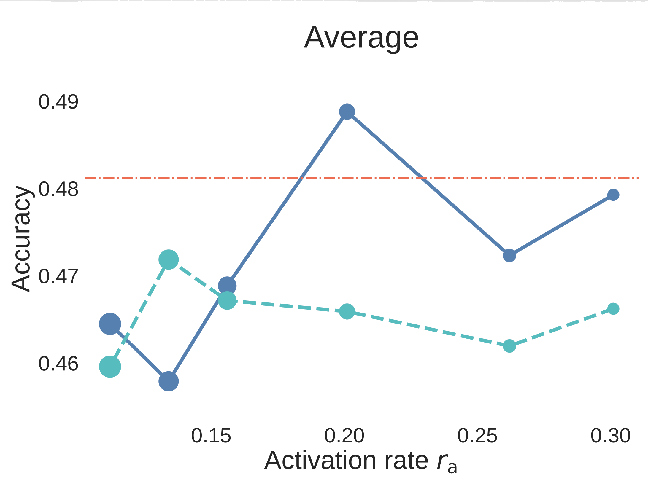
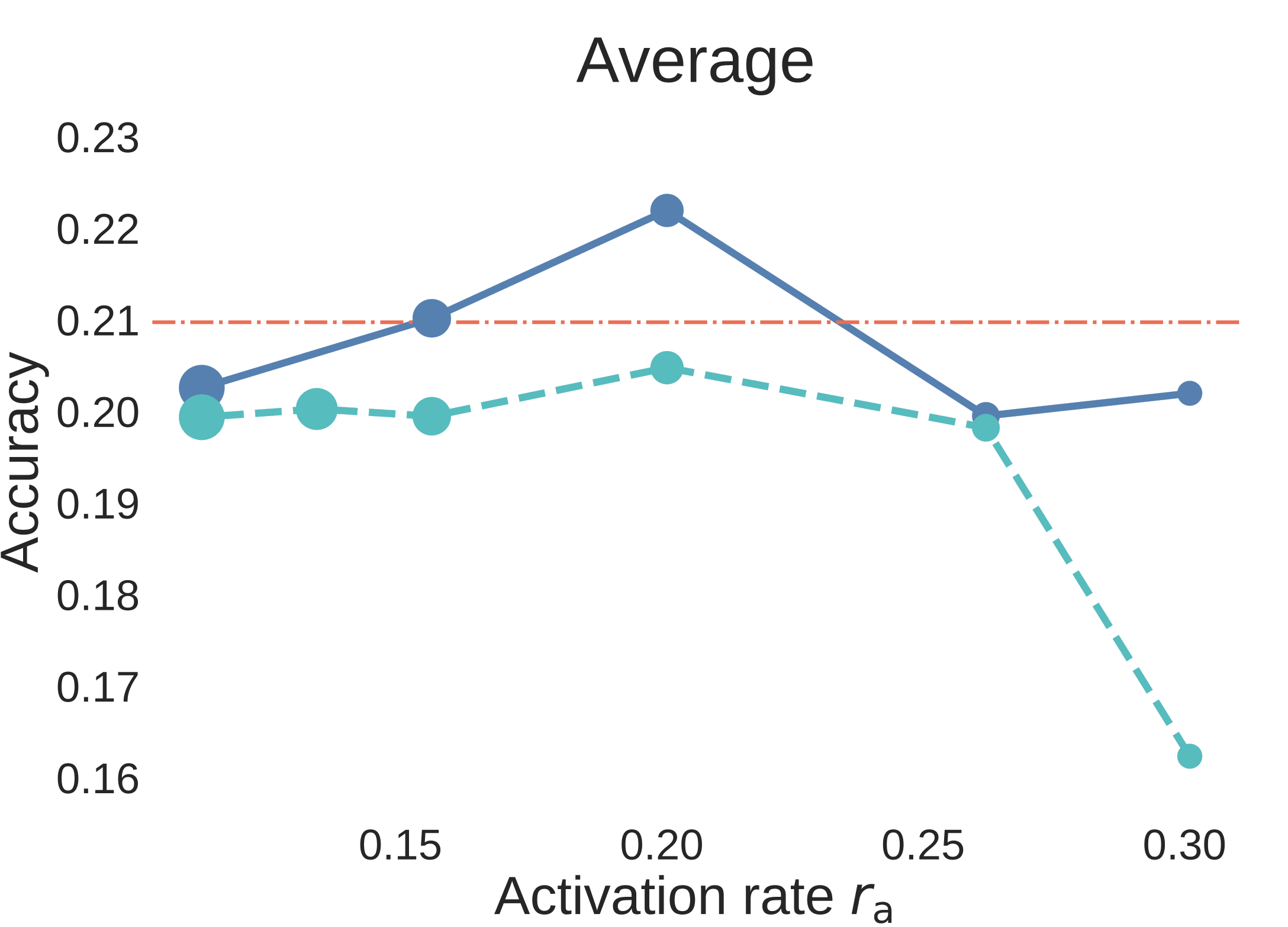
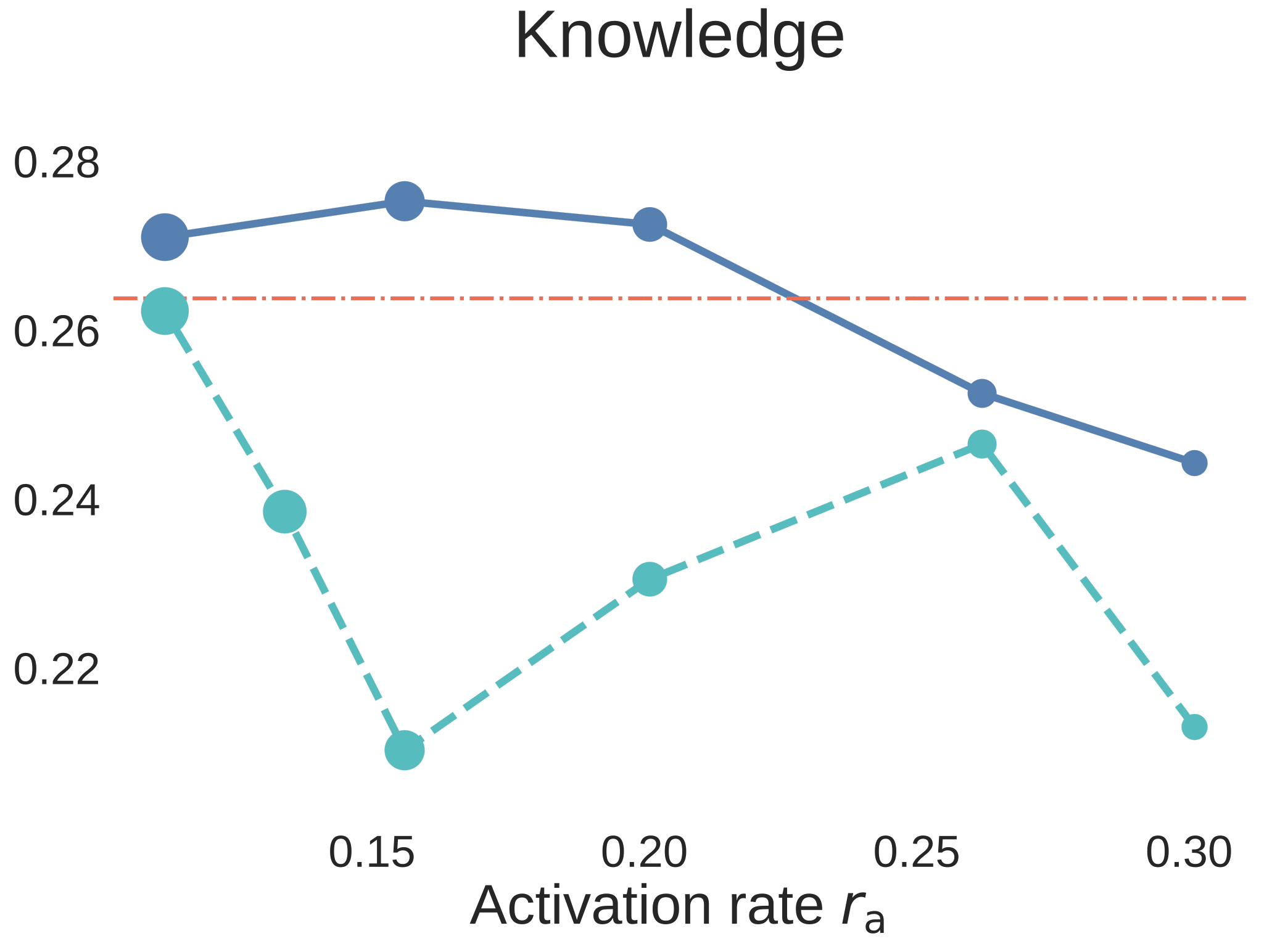
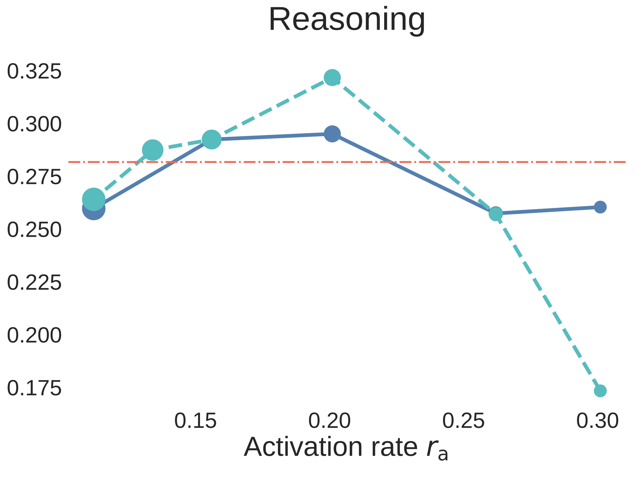
Figure 6. Step3C downstream evaluation for 7B aligned models. The blue solid curves use unique data, the cyan dashed curves use strict data reuse, and the red dash-dot line is the Dense-2C baseline. Unlike BPC plots, higher accuracy is better.
The result is not just “MoE wins on validation loss.” At , the MoE models remain strong after SFT, and the unique-data MoE is the clearest winner against the Dense comparison. The strict-reuse MoE remains competitive overall and is especially strong on reasoning, but the downstream curves expose an important capability split: data reuse has relatively little impact on reasoning, while knowledge-oriented benchmarks degrade more when unique tokens are reduced. In other words, for MoE, repeated data can strengthen reasoning, but it cannot fully replace missing world knowledge.
That makes Step3C more than a secondary check. It says the activation-rate sweet spot is relevant to aligned models too, and it clarifies where data reuse is most tolerable: more forgiving for reasoning, more dangerous for knowledge coverage.
8. Practical recipe and final takeaway
For teams building SOTA MoE LLMs, the guidance is sharper than “make it sparse.”
- MoE can match Dense with the same total parameters and training compute. Under the same total parameter count and the same training compute, the optimized MoE can match or surpass Dense. In these experiments, this means the first-order resource is training compute: once compute is matched, introducing sparsity does not create an inherent architectural disadvantage.
- The fundamental trade-off. In that regime, MoE trades higher consumed-token demand for much lower per-token FLOPs. At , the resource equation says to budget for roughly consumed tokens; the 7B sweet-spot row uses only
21.5%per-token FLOPs, roughly a5xinference-side FLOPs reduction at the same total-parameter footprint. - Scale-aware optimal sparsity. “Sparser is better” is the wrong instinct. Across the 2B, 3B, and 7B sweeps in this paper, the useful activation-rate region is broad but not arbitrary: roughly 10%-30%. As model size grows, this optimal activation-rate region may expand or shift toward sparser MoEs.
- Data reuse works, within limits. When unique data is limited, multi-epoch reuse can preserve the MoE advantage. In the 7B sweep, reuse within the moderate window remains useful; reasoning is relatively tolerant of repeated data, while knowledge coverage is more sensitive to unique tokens.
For example, suppose we want to train a 1T-total-parameter MoE model. A 1T Dense model would need about 20T tokens under the Chinchilla rule of thumb. If the MoE activates 100B parameters, or a 10% activation rate, then targeting Dense-level performance means budgeting for about 200T consumed tokens. If unique data is not enough, moderate multi-epoch reuse can help.
For teams training frontier models, this is the practical lesson: MoE scaling is not just a vague “sparse is efficient” story. It becomes a resource recipe: choose the right activation rate, use a more aggressive data scaling strategy, and when unique tokens are not enough, use data reuse moderately, for example within about three epochs.
Comments
Comments are powered by GitHub Discussions. Sign in with GitHub to join the thread.