Can We Train an MoE Model with the Same Total Parameters and Performance as Dense?

An ICLR 2026 Oral paper explainer: MoE needs a more aggressive data scaling strategy.

Appendix A. Detailed resource-equation derivation

This appendix gives the detailed derivation behind the resource equation, showing why, under the same total parameters and the same training compute, an MoE model needs to consume roughly $1/r_a$ times as many training tokens.

A.1 Fix the comparison first

We compare a Dense model and an MoE model under the same total non-embedding parameter count N. Let M denote per-token forward FLOPs, D denote consumed training tokens, and C denote total training compute. Training compute is approximated as:

$$C \approx 3MD. \tag{5}$$

where the factor 3 accounts for the usual forward-plus-backward cost. This factor will cancel when Dense and MoE are compared under equal C.

A.2 Dense: convert architecture shape into per-token FLOPs

For a Dense Transformer, Section 3 of the paper approximates the non-embedding parameter count as:

$$N_{\text{Dense}} \approx (4+3\alpha)D_m^2L = (4+3\alpha)\zeta^2L^3. \tag{6}$$

where D_m is model width, L is the number of layers, alpha = D_ffn / D_m, and zeta = D_m / L.

The corresponding per-token forward FLOPs are:

$$M_{\text{Dense}} \approx 2N_{\text{Dense}} + 4D_mSL = 2N_{\text{Dense}}\left(1+\frac{2\gamma_d}{4+3\alpha}\right). \tag{7}$$

The second equality comes from rewriting the attention term in units of N_Dense. Since:

$$D_m^2L \approx \frac{N_{\text{Dense}}}{4+3\alpha}, \qquad \gamma_d=\frac{S}{D_m}. \tag{8}$$

we have:

$$D_mSL = \frac{S}{D_m}D_m^2L = \gamma_dD_m^2L \approx \frac{\gamma_d}{4+3\alpha}N_{\text{Dense}}. \tag{9}$$

Therefore:

$$4D_mSL \approx \frac{4\gamma_d}{4+3\alpha}N_{\text{Dense}} = 2N_{\text{Dense}}\frac{2\gamma_d}{4+3\alpha}. \tag{10}$$

and:

$$2N_{\text{Dense}}+4D_mSL \approx 2N_{\text{Dense}}\left(1+\frac{2\gamma_d}{4+3\alpha}\right). \tag{11}$$

Here S is sequence length and gamma_d = S / D_m for the Dense model. The first term is the parameter-dominated Transformer computation; the second term is the attention sequence-length term. To keep the trade-off readable, group the shape-dependent multiplier into:

$$\kappa_{\text{Dense}} = 1+\frac{2\gamma_d}{4+3\alpha}. \tag{12}$$

So the Dense per-token FLOPs become:

$$M_{\text{Dense}} \approx 2N_{\text{Dense}}\kappa_{\text{Dense}}. \tag{13}$$

A.3 MoE: separate total parameters from activated parameters

For an MoE Transformer, total parameters and activated parameters are no longer the same. In the general setting where only some layers are MoE layers, the paper writes:

$$N_{\text{MoE}} \approx (4+3\mu)D_m^2L_e + (4+3\alpha)D_m^2L_d. \tag{14}$$ $$N_a \approx (4+3\beta)D_m^2L_e + (4+3\alpha)D_m^2L_d. \tag{15}$$

Here L_e is the number of MoE layers, L_d is the number of Dense layers, mu = (D_se + E D_e) / D_m, and beta = (D_se + K D_e) / D_m. The approximations omit small terms such as RMSNorm scale vectors, router/gate parameters, biases, and embedding parameters. The activation rate is:

$$r_a=\frac{N_a}{N_{\text{MoE}}}. \tag{16}$$

Using the same FLOPs convention as the Dense derivation, MoE per-token FLOPs are the activated-parameter computation plus the attention term:

$$M_{\text{MoE}} \approx 2N_a + 4D_mSL = 2r_aN_{\text{MoE}} + 4D_mSL. \tag{17}$$

For the simple all-MoE case used in the paper to expose the dependence on $r_a$, L_d = 0, so:

$$r_a \approx \frac{4+3\beta}{4+3\mu}. \tag{18}$$ $$M_{\text{MoE}} \approx 2r_aN_{\text{MoE}} \left(1+\frac{2\gamma_m}{4+3\beta}\right). \tag{19}$$

Define the MoE shape multiplier:

$$\kappa_{\text{MoE}} = 1+\frac{2\gamma_m}{4+3\beta}. \tag{20}$$

and the MoE per-token FLOPs become:

$$M_{\text{MoE}} \approx 2r_aN_{\text{MoE}}\kappa_{\text{MoE}}. \tag{21}$$

A.4 Equal total parameters gives the per-token compute ratio

We keep the total parameter count equal:

$$N_{\text{Dense}} = N_{\text{MoE}} = N. \tag{22}$$

Substitute the Dense and MoE FLOPs expressions:

$$R_c = \frac{M_{\text{MoE}}}{M_{\text{Dense}}} \approx r_a \frac{\kappa_{\text{MoE}}}{\kappa_{\text{Dense}}}. \tag{23}$$

Once architecture shape is fixed, kappa_Dense and kappa_MoE are approximately constants. Therefore the MoE/Dense per-token FLOPs ratio is nearly linear in $r_a$. This is exactly what Figure 1a empirically checks.

This is the inference-side bargain: smaller $r_a$ means fewer per-token FLOPs at the same total-parameter footprint.

A.5 Equal training compute forces the token multiplier

Now impose equal training compute:

$$3M_{\text{Dense}}D_{\text{Dense}} \approx 3M_{\text{MoE}}D_{\text{MoE}}. \tag{24}$$

Cancel the factor 3 and rearrange:

$$\frac{D_{\text{MoE}}}{D_{\text{Dense}}} \approx \frac{M_{\text{Dense}}}{M_{\text{MoE}}} = \frac{1}{R_c} \approx \frac{1}{r_a} \frac{\kappa_{\text{Dense}}}{\kappa_{\text{MoE}}}. \tag{25}$$

When the shape multipliers are fixed and comparable, the dominant scaling is:

$$\frac{D_{\text{MoE}}}{D_{\text{Dense}}} \propto \frac{1}{r_a}. \tag{26}$$

This is the mathematical reason behind the blog’s central claim: at fixed total parameters and fixed training compute, MoE pays for lower per-token FLOPs by consuming roughly $1/r_a$ times more training tokens.

A.6 Why Step 1 must come before the activation-rate sweep

The main reason is fairness to the MoE side. Before comparing MoE with a tuned Dense baseline, the paper first has to give MoE a reasonably optimized architecture; otherwise a weak result could simply mean that the MoE backbone was poorly chosen. Step 1 therefore searches the layer arrangement, shared experts, routing/top-K choices, expert allocation, and shape ratios to establish a strong MoE backbone.

Once that backbone is fixed, the later activation-rate sweep gains an additional benefit: kappa_MoE and other shape factors are no longer changing with every $r_a$ point, so the sweep is cleaner. But this is secondary. The primary reason for Step 1 is to compare Dense against the best-performing MoE configuration the study can identify, rather than against an under-optimized sparse model.

Appendix B. Related work notes

B.1 DeepSeekMoE and DeepSeek-V2

DeepSeekMoE 16B vs 7B Dense is a typical example of the first comparison style. The paper scales DeepSeekMoE to 16B total parameters and trains it on a 2T-token corpus. It reports that DeepSeekMoE 16B achieves comparable performance to Dense DeepSeek 7B, which was trained on the same 2T corpus, while using only about 40% of the computations. It also reports comparable performance to LLaMA2 7B, which has about 2.5x the activated parameters [1].

This is a strong active-compute efficiency result, but it is not an equal-total-parameter comparison: the MoE has 16B total parameters, while the Dense reference has 7B. The result therefore answers whether a sparse model can be highly compute-efficient when it is allowed a larger total expert reservoir. It does not directly answer whether an MoE model can match a Dense model when total parameters N are held equal. DeepSeek-V2 later scales the same general sparse-MoE direction to 236B total parameters and 21B activated parameters [2], reinforcing the engineering value of the line while also illustrating why total-parameter control matters.

B.2 Kimi K2 sparsity scaling

Kimi K2 provides a clear example of the second comparison style. In its sparsity scaling law experiment, it fixes 8 activated experts and 1 shared expert, then varies the total number of experts to create sparsity levels from 8 to 64. The report states that increasing sparsity consistently lowers both training and validation loss, and Kimi K2 adopts sparsity 48, activating 8 out of 384 experts per forward pass [3].

Again, this is a useful result, but it is not an equal-total-parameter Dense-vs-MoE comparison. The experiment fixes active expert count / per-token compute, not total parameters; it allows the total expert pool, and therefore total parameters, to grow.

Appendix C. Step 1 architecture-search evidence

This appendix expands the Step 1 architecture search and explains how the paper narrows the MoE design space before running the activation-rate sweep.

C.1 Layer arrangement and shared experts

The paper first tests how to arrange Dense and MoE layers. The shared hyperparameters are D_m = 1408, D_ffn = 3904, and Norm = True. The experiments compare full, interleave, 1dense, and shared-expert variants.

Table 4. Experimental settings and results for MoE layer arrangement and shared experts.

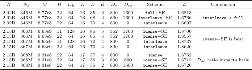
Table 4 has three useful readings. First, in the initial group, interleave improves over full (1.6766 or 1.6697 vs. 1.6813 training loss). Second, in the larger comparison group, 1dense+SE is the strongest setting, with 1.8557 beating the corresponding interleave rows (1.8737 and 1.8620). Third, changing the shared-expert ratio has only a small effect in the final group (1.6752, 1.6712, and 1.6726). This is why the paper continues with 1dense+SE and sets D_se = K D_e.

C.2 Gate score normalization

The gate-normalization experiment uses Scheme = 1dense, L = 17, D_m = 1408, D_ffn = 3904, H = 22, and D_h = 64.

Table 5. Experimental settings and results for gate score normalization.

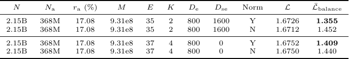
Table 5 shows that the loss difference is small in these small-model ablations: with shared experts, normalization gives 1.6726 vs. 1.6712 without normalization; without shared experts, it gives 1.6752 vs. 1.6750. The clearer effect is on balance loss: normalization reduces average balance loss from 1.452 to 1.355 in the shared-expert setting, and from 1.440 to 1.409 in the no-shared-expert setting.

The right interpretation is a limitation of the paper, not a general recommendation to avoid normalization. Follow-up experiments at larger sizes show normalization is significantly better than no normalization. For extrapolation, normalized routing should be preferred. Turning normalization off does not change the paper’s conclusions in the small-model setting, but it should not be treated as the best large-scale recipe.

C.3 Top-K routing and expert granularity

The top-K experiment fixes Scheme = 1dense, L = 16, D_m = 1408, D_ffn = 3904, H = 11, D_h = 128, and Norm = False. It varies K and expert size across several activation-rate regions.

Table 6. Experimental settings and results for top-K routing.

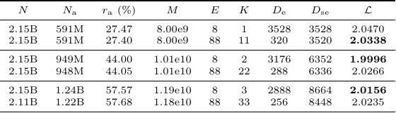
Table 6 supports a bounded conclusion rather than a single universal K. At $r_a \approx 27\%$, K = 11 performs better than K = 1 (2.0338 vs. 2.0470). At higher activation rates, much larger K values are worse than smaller ones: K = 2 beats K = 22 at $r_a \approx 44\%$ (1.9996 vs. 2.0266), and K = 3 beats K = 33 at $r_a \approx 58\%$ (2.0156 vs. 2.0235). The paper’s practical decision is therefore to avoid both K = 1 and overly large K whenever possible.

C.4 Shape-ratio search

Finally, the paper explores shape ratios under Scheme = 1dense, S = 16384, and D_h = 128. The full table is in the paper appendix; Figure 7 summarizes the trend.

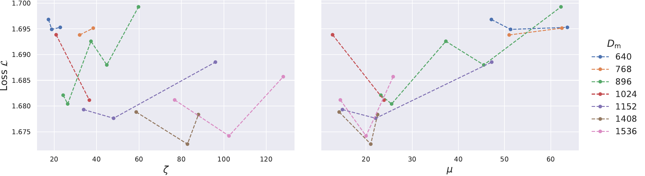
Figure 7. Shape-ratio search over zeta = D_m / L and mu = (D_se + E D_e) / D_m.

The paper explicitly notes that performance fluctuates substantially for a given zeta or mu, so this search is not presented as a precise scaling law. The more robust reading is a range-level conclusion: zeta in roughly 60-120 is a reasonable region, while mu around 20 is a reasonable region. The later activation-rate experiments should therefore be understood as using a representative setting inside this reasonable backbone region, not as proving that zeta = 88 and mu = 22 are uniquely optimal.

Appendix D. Notation

Table 7 follows the paper’s notation table, with two extra shorthand terms used in this blog.

Table 7. Notation used in the paper and this blog.

Symbol	Definition	Symbol	Definition
$D$	Dataset size / consumed training tokens.	$M$	Compute per token in FLOPs, excluding embeddings.
$C$	Total training compute in FLOPs, approximately $M \cdot D$.	$N$	Number of non-vocabulary / non-embedding parameters.
$N_a$	Number of activated parameters.	$r_a$	Activation rate, $N_a/N$.
$L_e$	Number of MoE layers.	$L_d$	Number of Dense layers.
$L$	Total number of layers, $L_e + L_d$.	$\alpha$	FFN expansion ratio, $D_{\text{ffn}}/D_m$.
$\zeta$	Model aspect ratio, $D_m/L$.	$\gamma$	Sequence-to-width ratio, $S/D_m$.
$S$	Sequence length.	$H$	Number of attention heads.
$D_m$	Model hidden dimension.	$D_{\text{ffn}}$	FFN hidden dimension.
$D_h$	Dimension of each attention head.	$D_e$	Expert hidden dimension.
$D_{\text{se}}$	Shared-expert hidden dimension.	$E$	Number of experts.
$K$	Number of chosen experts.	$\beta$	Activated FFN-to-model ratio in MoE layers, $(D_{\text{se}}+KD_e)/D_m$.
$\mu$	Total FFN-to-model ratio in MoE layers, $(D_{\text{se}}+ED_e)/D_m$.	$\kappa_{\text{Dense}}$, $\kappa_{\text{MoE}}$, $R_c$	Blog shorthand for shape multipliers and per-token FLOPs ratio, $R_c=M_{\text{MoE}}/M_{\text{Dense}}$.

Appendix E. Pretraining data recipe and downstream-score interpretation

Table 8 reproduces the paper’s Appendix Table 3, which reports the pretraining mixture for reproducibility and compares it with the LLaMA-1 recipe [4]. Table 8 is important for interpreting downstream results: the study intentionally uses a simple, LLaMA-1-style mixture rather than a modern domain-boosted recipe.

Table 8. Paper Table 3: pretraining data recipe compared with the LLaMA-1 recipe.

Dataset class	Our recipe	Our dataset detail	LLaMA-1 recipe	LLaMA-1 dataset detail	Diff
WebData-en	79.53%	CC (English)	82.00%	67% CC + 15% C4 (English)	-2.47%
Code	4.62%	The Stack	4.50%	Github-Big Query	+0.12%
Wikipedia	5.06%	en: 1.69%, cn: 0.13%, others: 3.24%	4.50%	multi-lingual	+0.56%
Book	5.18%	open-source English books	4.50%	Book3, Gutenberg	+0.68%
arXiv	3.38%	as class name	1.06%	as class name	+2.32%
StackExchange	2.21%	as class name	2.00%	as class name	+0.21%

This data choice also explains how to read the downstream scores. Our goal is not to maximize absolute benchmark numbers with a modern domain-boosted recipe, but to compare Dense and MoE under the same controlled pretraining mixture. Because the corpus is close to LLaMA-1, with roughly 80% generic web data and only 4.62% explicit code data, high-purity math/code/knowledge content is not dense in the training data. Therefore, absolute Math/Code/knowledge numbers should not be read as the paper’s main target.

Appendix F. Limitations and discussion

There are four limitations worth stating directly.

First, the data mixture is a product of the time when the experiments were designed. The work was carried out around the 2024 pretraining-recipe regime, and the corpus was intentionally close to LLaMA-1 so that the 7B Dense baseline could be interpreted against a familiar reference. This makes the controlled Dense-vs-MoE comparison cleaner, but it also means the absolute downstream scores are not what we would expect from a modern data recipe. If we ran this study today, we would add a controlled high-quality annealing stage so that more downstream benchmarks could be used as direct capability probes. That design is not trivial, especially because MoE and Dense consume different numbers of tokens under equal compute, so the unique-token accounting would have to be handled carefully. Still, the limitation mostly affects downstream absolute scores, not the central MoE data-per-token-FLOPs trade-off.

Second, some architecture choices are dated. The models use choices such as ALiBi positional encoding, reflecting the period in which the experiments were launched. Gate normalization should also be read this way: in the paper’s small-model ablations, normalization mainly reduces balance loss and has little effect on loss, but later larger-scale experiments show normalized routing is clearly better. For extrapolating the recipe, normalized routing should be preferred. This does not undermine the paper’s main conclusion, because the small-model result is internally controlled and the normalization choice does not drive the observed activation-rate trade-off.

Third, the architecture search is greedy. The paper first searches for a strong MoE backbone, then fixes it and sweeps $r_a$. This saves a large amount of compute and makes the sweep cleaner by keeping shape factors such as $\kappa_{\text{MoE}}$ more stable. The limitation is that different activation rates may have different optimal architectures. The ideal experiment would run a fresh architecture search for every $r_a$, but that adds another experimental dimension and would make the cost grow roughly like the product of the architecture grid and the activation-rate grid. Our later check around the 13% activation-rate point suggests that re-searching the architecture can improve sparse points and bring them closer to the Dense baseline, but it still did not surpass the roughly 20% $r_a$ point. So this limitation may shift the exact optimal region, but it is unlikely to remove the existence of an optimal activation-rate region.

Fourth, the scale only reaches 7B. The 7B ablations are carefully controlled: different-sparsity MoE models keep the same layer count $L$ and hidden dimension $D_m$, so effective depth and information-channel width are held fixed. Since MoE sparsity is governed mainly by $\beta$ and $\mu$, not by $L$ or $D_m$, fixing $N$, $L$, and $D_m$ largely fixes $\mu$ and lets the sweep adjust $r_a$ through $\beta$. This is a rigorous control-variable design. But it also means that very sparse models may fail partly because $\beta$ becomes too small and turns the activated FFN capacity into a bottleneck.

The scale issue is easiest to see by reusing the parameterization in Appendix A instead of deriving it again. Eq. (14) gives the MoE total-parameter approximation, and Eq. (18) gives the simple activation-rate form after imposing the all-MoE condition $L_d=0$. The approximation sign matters: these formulas intentionally ignore small terms such as RMSNorm scale vectors, router/gate parameters, biases, and embedding parameters.

Now keep $L$, $D_m$, $L_e$, and $L_d$ comparable while scaling total parameters from 7B to 14B. Eq. (14) says that, once the Dense-layer term and the depth/width terms are mostly fixed, the extra parameters mainly have to enter through the MoE FFN reservoir, i.e., through $\mu$. In the pure $L_d=0$ case, $N_{\text{MoE}} \approx (4+3\mu)D_m^2L_e$, so doubling $N_{\text{MoE}}$ roughly doubles $(4+3\mu)$ and makes $\mu$ close to $2\times$ larger when $\mu$ is already large. With a small fixed Dense-layer term, this becomes an approximation rather than an equality, but the direction is the same.

The corresponding statement about $\beta$ follows directly from Eq. (18). Under the same $L_d=0$ condition:

$$\begin{aligned} r_a(4+3\mu) &\approx 4+3\beta,\\ 3\beta &\approx 3r_a\mu + 4r_a - 4,\\ \beta &\approx r_a\mu + \frac{4}{3}(r_a-1). \end{aligned} \tag{27}$$

When $\mu$ is large enough, the constant offset $\frac{4}{3}(r_a-1)$ is less important than the $r_a\mu$ term. Therefore, if $\mu$ becomes roughly $2\times$ larger, $\beta$ also becomes roughly $2\times$ larger at the same $r_a$. This means the same activation rate can correspond to a much wider activated FFN path at larger total scale, making the low-$\beta$ bottleneck less severe. For this reason, we expect the useful activation-rate region may expand or move toward sparser MoEs at larger scale. This is an important open question beyond the paper’s compute budget, but it does not change the core answer: an MoE can match Dense at the same total-parameter scale, but it must pay with more consumed tokens, and it is not optimal simply because it is made as sparse as possible.

---

---

References / 参考文献

[1] Dai, D. et al. (2024). DeepSeekMoE: Towards Ultimate Expert Specialization in Mixture-of-Experts Language Models. arXiv:2401.06066. Local PDF: references/deepseekmoe-2401.06066.pdf.

[2] DeepSeek-AI et al. (2024). DeepSeek-V2: A Strong, Economical, and Efficient Mixture-of-Experts Language Model. arXiv:2405.04434. Local PDF: references/deepseek-v2-2405.04434.pdf.

[3] Kimi Team et al. (2025). Kimi K2: Open Agentic Intelligence. arXiv:2507.20534. Local PDF: references/kimi-k2-2507.20534.pdf.

[4] Touvron, H. et al. (2023). LLaMA: Open and Efficient Foundation Language Models. arXiv:2302.13971.