能否训出和 Dense 总参相同、性能相同的 MoE 模型？

ICLR 2026 Oral Paper的解读：MoE 需要更加激进的 Data Scaling 策略

附录 A：资源方程的详细推导

本章节详细展开资源方程的推导，说明为什么在 same total parameters 和 same training compute 下，MoE 需要消耗大约 $1/r_a$ 倍 training tokens。

A.1 先固定比较对象

比较对象先固定：Dense model 和 MoE model 拥有相同的 total non-embedding parameter count N。令 M 表示 per-token forward FLOPs，D 表示 consumed training tokens，C 表示 total training compute。训练算力近似为：

$$C \approx 3MD. \tag{5}$$

这里的系数 3 对应常见的 forward-plus-backward cost。做 equal-C 比较时，这个系数会在 Dense 和 MoE 两边抵消。

A.2 Dense：把 architecture shape 写进 per-token FLOPs

对 Dense Transformer，论文第 3 节把 non-embedding parameter count 近似为：

$$N_{\text{Dense}} \approx (4+3\alpha)D_m^2L = (4+3\alpha)\zeta^2L^3. \tag{6}$$

其中 D_m 是 model width，L 是 layers 数量，alpha = D_ffn / D_m，zeta = D_m / L。

对应的 per-token forward FLOPs 为：

$$M_{\text{Dense}} \approx 2N_{\text{Dense}} + 4D_mSL = 2N_{\text{Dense}}\left(1+\frac{2\gamma_d}{4+3\alpha}\right). \tag{7}$$

第二个等号的关键，是把 attention term 改写到 N_Dense 的量纲下。由于：

$$D_m^2L \approx \frac{N_{\text{Dense}}}{4+3\alpha}, \qquad \gamma_d=\frac{S}{D_m}. \tag{8}$$

可以得到：

$$D_mSL = \frac{S}{D_m}D_m^2L = \gamma_dD_m^2L \approx \frac{\gamma_d}{4+3\alpha}N_{\text{Dense}}. \tag{9}$$

因此：

$$4D_mSL \approx \frac{4\gamma_d}{4+3\alpha}N_{\text{Dense}} = 2N_{\text{Dense}}\frac{2\gamma_d}{4+3\alpha}. \tag{10}$$

也就是：

$$2N_{\text{Dense}}+4D_mSL \approx 2N_{\text{Dense}}\left(1+\frac{2\gamma_d}{4+3\alpha}\right). \tag{11}$$

这里 S 是 sequence length，gamma_d = S / D_m。第一项来自 parameter-dominated Transformer computation，第二项来自 attention 的 sequence-length term。为了让后面的 trade-off 更清楚，把这些 shape-dependent multiplier 合并为：

$$\kappa_{\text{Dense}} = 1+\frac{2\gamma_d}{4+3\alpha}. \tag{12}$$

于是 Dense 的 per-token FLOPs 可以写成：

$$M_{\text{Dense}} \approx 2N_{\text{Dense}}\kappa_{\text{Dense}}. \tag{13}$$

A.3 MoE：区分 total parameters 和 activated parameters

到 MoE Transformer，total parameters 和 activated parameters 就分开了。在只有部分层是 MoE layers 的一般设定下，论文写成：

$$N_{\text{MoE}} \approx (4+3\mu)D_m^2L_e + (4+3\alpha)D_m^2L_d. \tag{14}$$ $$N_a \approx (4+3\beta)D_m^2L_e + (4+3\alpha)D_m^2L_d. \tag{15}$$

这里 L_e 是 MoE layers 数量，L_d 是 Dense layers 数量，mu = (D_se + E D_e) / D_m，beta = (D_se + K D_e) / D_m。这些近似会忽略 RMSNorm scale vectors、router/gate parameters、bias、embedding parameters 等小项。Activation rate 定义为：

$$r_a=\frac{N_a}{N_{\text{MoE}}}. \tag{16}$$

沿用 Dense 推导中的 FLOPs convention，MoE 的 per-token FLOPs 由 activated-parameter computation 加 attention term 构成：

$$M_{\text{MoE}} \approx 2N_a + 4D_mSL = 2r_aN_{\text{MoE}} + 4D_mSL. \tag{17}$$

为了把 $r_a$ 的作用单独拎出来，论文用一个简单的 all-MoE case 来说明。此时 L_d = 0，所以：

$$r_a \approx \frac{4+3\beta}{4+3\mu}. \tag{18}$$ $$M_{\text{MoE}} \approx 2r_aN_{\text{MoE}} \left(1+\frac{2\gamma_m}{4+3\beta}\right). \tag{19}$$

定义 MoE 的 shape multiplier：

$$\kappa_{\text{MoE}} = 1+\frac{2\gamma_m}{4+3\beta}. \tag{20}$$

则 MoE 的 per-token FLOPs 为：

$$M_{\text{MoE}} \approx 2r_aN_{\text{MoE}}\kappa_{\text{MoE}}. \tag{21}$$

A.4 Equal total parameters 给出 per-token compute ratio

我们保持总参一致：

$$N_{\text{Dense}} = N_{\text{MoE}} = N. \tag{22}$$

代入 Dense 和 MoE 的 FLOPs 表达式：

$$R_c = \frac{M_{\text{MoE}}}{M_{\text{Dense}}} \approx r_a \frac{\kappa_{\text{MoE}}}{\kappa_{\text{Dense}}}. \tag{23}$$

当 architecture shape 固定后，kappa_Dense 和 kappa_MoE 可以近似看作常数。因此，MoE/Dense per-token FLOPs ratio 会基本跟着 $r_a$ 线性变化。图 1a 经验上检查的正是这一点。

这就是 inference 侧的账：在相同 total-parameter footprint 下，$r_a$ 越小，per-token FLOPs 越接近 activation-rate 量级。

A.5 Equal training compute 推出 token multiplier

再加入 equal training compute：

$$3M_{\text{Dense}}D_{\text{Dense}} \approx 3M_{\text{MoE}}D_{\text{MoE}}. \tag{24}$$

消去系数 3 并整理：

$$\frac{D_{\text{MoE}}}{D_{\text{Dense}}} \approx \frac{M_{\text{Dense}}}{M_{\text{MoE}}} = \frac{1}{R_c} \approx \frac{1}{r_a} \frac{\kappa_{\text{Dense}}}{\kappa_{\text{MoE}}}. \tag{25}$$

当 shape multipliers 被固定且量级可比时，主导项就是：

$$\frac{D_{\text{MoE}}}{D_{\text{Dense}}} \propto \frac{1}{r_a}. \tag{26}$$

这就是正文核心 claim 的数学来源：在 fixed total parameters 和 fixed training compute 下，MoE 用大约 $1/r_a$ 倍 training tokens，换取约 $r_a$ 倍的 per-token FLOPs。

A.6 为什么 Step 1 必须在 activation-rate sweep 之前

主要原因是要对 MoE 侧公平。拿 MoE 和调好的 Dense baseline 比之前，论文必须先给 MoE 一个合理优化过的 architecture；否则，差结果可能只是 MoE backbone 没选好。Step 1 因此搜索 layer arrangement、shared experts、routing/top-K choices、expert allocation 和 shape ratios，用来建立一个 strong MoE backbone。

Backbone 固定之后，还有一个额外好处：kappa_MoE 和其他 shape factors 不会随着每个 $r_a$ 点一起变化，所以 sweep 更干净。但这不是主因。Step 1 的主因是让 Dense 去和这项研究能找到的最佳 MoE configuration 比较，而不是和一个 under-optimized sparse model 比较。

附录 B：相关工作说明

B.1 DeepSeekMoE 和 DeepSeek-V2

DeepSeekMoE 16B vs 7B Dense 是第一类比较方式里典型的例子。DeepSeekMoE 论文把 MoE 扩到 16B total parameters，并在 2T-token corpus 上训练。论文报告 DeepSeekMoE 16B 能达到与同样使用 2T corpus 训练的 Dense DeepSeek 7B 可比的性能，同时只用约 40% computation；它也能达到与 LLaMA2 7B 可比的表现，而 LLaMA2 7B 的 activated parameters 大约是它的 2.5x [1]。

这是很强的 active-compute efficiency 结果，但它不是 equal-total-parameter comparison：MoE 有 16B total parameters，而 Dense reference 是 7B。所以它回答的是：当 sparse model 可以使用更大的 total expert reservoir 时，能不能做到很高的 compute efficiency。它没有直接回答 total parameters N 固定时，MoE 能否追平 Dense。DeepSeek-V2 后续把同一类 sparse-MoE 路线扩展到 236B total parameters / 21B activated parameters [2]，进一步说明这条路线的工程价值，也说明为什么需要控制 total parameters。

B.2 Kimi K2 sparsity scaling

Kimi K2 是第二类比较方式的清楚例子。在 sparsity scaling law experiment 中，它固定 8 个 activated experts 和 1 个 shared expert，通过改变 total experts 数量构造 sparsity 8 到 64 的模型。报告显示，increasing sparsity 会持续降低 training 和 validation loss；最终 Kimi K2 采用 sparsity 48，每次 forward 在 384 个 experts 中激活 8 个 [3]。

这个结果同样有价值，但它也不是 equal-total-parameter Dense-vs-MoE comparison。实验固定的是 active expert count / per-token compute，而不是 total parameters；它允许 total expert pool 增长，也就是 total parameters 增长。

附录 C：Step 1 architecture-search evidence

这个附录展开 Step 1 architecture search，说明论文如何在 activation-rate sweep 之前先收窄 MoE 的设计空间。

C.1 Layer arrangement and shared experts

论文首先测试 Dense 和 MoE layers 怎么排。共同超参数是 D_m = 1408、D_ffn = 3904、Norm = True。实验比较 full、interleave、1dense 以及 shared-expert variants。

表 4. MoE layer arrangement 和 shared experts 的实验设置与结果。

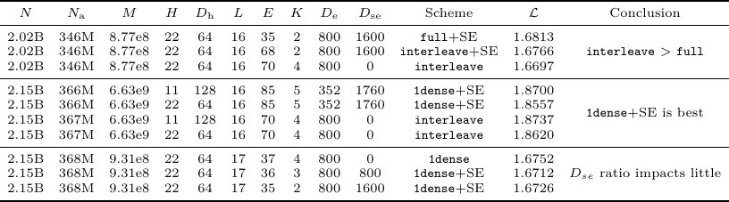
表 4 可以分三层读。第一，初始组里，interleave 优于 full（training loss 1.6766 或 1.6697 vs. 1.6813）。第二，更大的比较组里，1dense+SE 是最强设置，1.8557 优于对应的 interleave rows（1.8737 和 1.8620）。第三，最后一组里，shared-expert ratio 的影响很小（1.6752、1.6712、1.6726）。因此论文后续采用 1dense+SE，并设置 D_se = K D_e。

C.2 Gate score normalization

Gate-normalization 实验使用 Scheme = 1dense、L = 17、D_m = 1408、D_ffn = 3904、H = 22、D_h = 64。

表 5. Gate score normalization 的实验设置与结果。

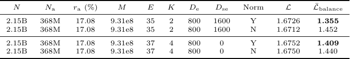
表 5 显示，在这些小模型 ablations 中，loss 差异很小：有 shared experts 时，normalization 是 1.6726，no normalization 是 1.6712；没有 shared experts 时，对应是 1.6752 vs. 1.6750。更清楚的影响体现在 balance loss：有 shared-expert setting 中，normalization 将 average balance loss 从 1.452 降到 1.355；无 shared-expert setting 中，从 1.440 降到 1.409。

这里要直接承认 limitation：这不是一个“应该避免 normalization”的通用建议。后续更大尺度实验显示 normalization 显著优于 no normalization。外推到更大模型时，应优先使用 normalized routing。关闭 normalization 不改变本文在小模型 setting 下的结论，但不应该被当作 large-scale recipe。

C.3 Top-K routing and expert granularity

Top-K 实验固定 Scheme = 1dense、L = 16、D_m = 1408、D_ffn = 3904、H = 11、D_h = 128、Norm = False，并在几个 activation-rate regions 中改变 K 和 expert size。

表 6. Top-K routing 的实验设置与结果。

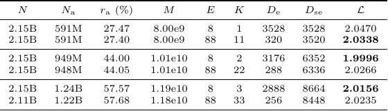
表 6 支持的是有边界的结论，而不是某个 universal K。在 $r_a \approx 27\%$ 时，K = 11 优于 K = 1（2.0338 vs. 2.0470）。在更高 activation rates 下，过大的 K 反而不如小一些的 K：$r_a \approx 44\%$ 时 K = 2 优于 K = 22（1.9996 vs. 2.0266），$r_a \approx 58\%$ 时 K = 3 优于 K = 33（2.0156 vs. 2.0235）。因此论文的实践选择是：尽可能避免 K = 1，也避免过大的 K。

C.4 Shape-ratio search

最后，论文在 Scheme = 1dense、S = 16384、D_h = 128 下搜索 shape ratios。完整表格在论文 appendix 中；图 7 总结了这个趋势。

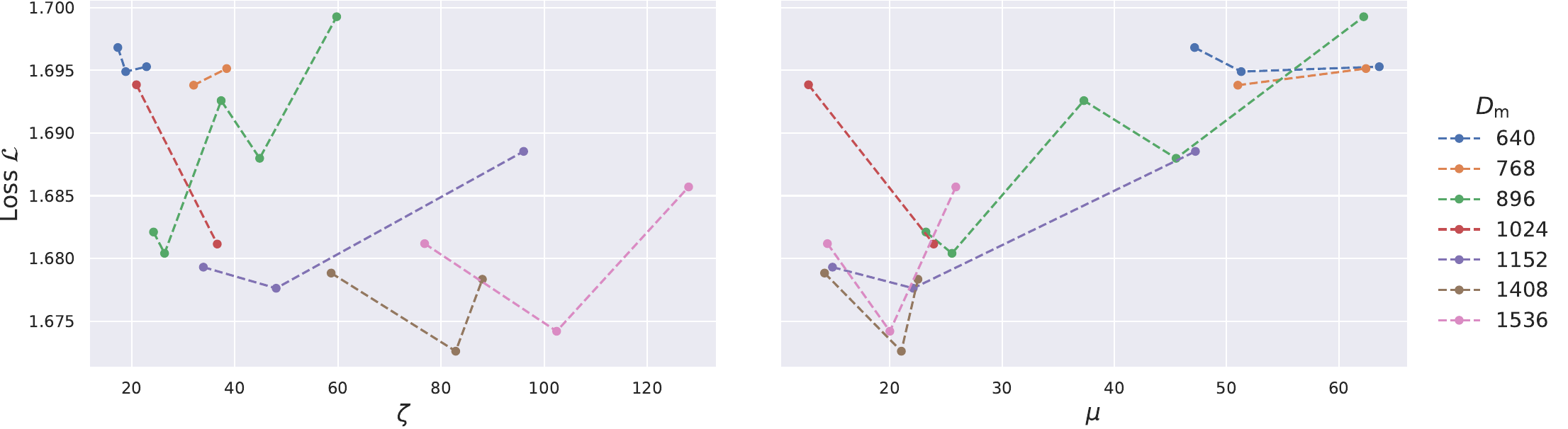
图 7. 对 zeta = D_m / L 和 mu = (D_se + E D_e) / D_m 的 shape-ratio search。

论文明确说明：固定某个 zeta 或 mu 时，performance fluctuation 仍然明显，所以这里不应被解读为精确 scaling law。更稳妥的读法是区间级结论：zeta 在约 60-120 是合理范围，mu 在 20 左右是合理范围。后续 activation-rate experiments 应理解为在这个合理 backbone region 内选了一个代表性设置，而不是证明 zeta = 88 和 mu = 22 是唯一最优点。

附录 D：Notation

表 7 参考论文 notation table，并补充正文博客中额外使用的两个 shorthand。

表 7. 论文和本文使用的 notation。

Symbol	Definition	Symbol	Definition
$D$	Dataset size / consumed training tokens。	$M$	Per-token FLOPs，不含 embedding。
$C$	Total training compute，近似为 $M \cdot D$。	$N$	Non-vocabulary / non-embedding parameters。
$N_a$	Activated parameters。	$r_a$	Activation rate，$N_a/N$。
$L_e$	MoE layers 数量。	$L_d$	Dense layers 数量。
$L$	总层数，$L_e + L_d$。	$\alpha$	FFN expansion ratio，$D_{\text{ffn}}/D_m$。
$\zeta$	Model aspect ratio，$D_m/L$。	$\gamma$	Sequence-to-width ratio，$S/D_m$。
$S$	Sequence length。	$H$	Attention heads 数量。
$D_m$	Model hidden dimension。	$D_{\text{ffn}}$	FFN hidden dimension。
$D_h$	Attention head dimension。	$D_e$	Expert hidden dimension。
$D_{\text{se}}$	Shared-expert hidden dimension。	$E$	Experts 数量。
$K$	Number of chosen experts。	$\beta$	MoE layers 中的 activated FFN-to-model ratio，$(D_{\text{se}}+KD_e)/D_m$。
$\mu$	MoE layers 中的 total FFN-to-model ratio，$(D_{\text{se}}+ED_e)/D_m$。	$\kappa_{\text{Dense}}$, $\kappa_{\text{MoE}}$, $R_c$	博客中的 shorthand：shape multipliers 和 per-token FLOPs ratio，$R_c=M_{\text{MoE}}/M_{\text{Dense}}$。

附录 E：Pretraining data recipe and downstream-score interpretation

表 8 复现了论文 Appendix Table 3 的 pretraining mixture，并和 LLaMA-1 recipe 做了对比 [4]。表 8 对理解 downstream results 很重要：本文有意使用简单的 LLaMA-1-style mixture，而不是现代工业模型常用的 domain-boosted recipe。

表 8. 论文 Table 3：pretraining data recipe compared with the LLaMA-1 recipe。

Dataset class	Our recipe	Our dataset detail	LLaMA-1 recipe	LLaMA-1 dataset detail	Diff
WebData-en	79.53%	CC (English)	82.00%	67% CC + 15% C4 (English)	-2.47%
Code	4.62%	The Stack	4.50%	Github-Big Query	+0.12%
Wikipedia	5.06%	en: 1.69%, cn: 0.13%, others: 3.24%	4.50%	multi-lingual	+0.56%
Book	5.18%	open-source English books	4.50%	Book3, Gutenberg	+0.68%
arXiv	3.38%	as class name	1.06%	as class name	+2.32%
StackExchange	2.21%	as class name	2.00%	as class name	+0.21%

这个数据选择也决定了 downstream scores 应该如何解读。我们的目标不是用现代 domain-boosted recipe 去最大化绝对 benchmark 分数，而是在同一套受控 pretraining mixture 下比较 Dense 和 MoE。由于这套 corpus 接近 LLaMA-1，约 80% 是 generic web data，显式 code data 只有 4.62%，高纯度 math/code/knowledge 内容在训练数据中并不密集。因此，Math/Code/knowledge 的绝对分数不应被看作这篇论文的主要目标。

附录 F：Limitation and Discussion

这里有四个 limitation 需要直接说明。

第一，数据配比有时代限制。这个工作的实验设计发生在 2024 年前后的 pretraining recipe 语境里；为了让 7B Dense baseline 能和 LLaMA-1 7B 有可解释的参照，论文使用了接近 LLaMA-1 的数据配比。这样做让 Dense-vs-MoE 的 controlled comparison 更干净，但也导致 downstream benchmark 的绝对分数不够现代。如果今天重新做，我会加入受控的 high-quality annealing stage，让更多 downstream benchmark 能直接成为 MoE 和 Dense 能力差异的观测窗口。不过这个操作并不简单，尤其是在 MoE 和 Dense 的 consumed tokens、unique tokens 不完全相同的情况下，数据账必须重新设计得非常干净。因此，这个 limitation 主要影响 downstream 绝对分数，不影响本文最核心的 MoE data-per-token-FLOPs trade-off 结论。

第二，部分 architecture choice 也有时代限制。模型使用了 ALiBi positional encoding 等现在看来偏旧的设计。Gate normalization 也应该放在这个语境下理解：在本文的小模型 ablation 中，normalization 主要降低 balance loss，对 loss 本身影响很小；但后续更大尺度实验显示 normalized routing 明显更好。因此如果外推本文 recipe 到更大模型，应该优先使用 normalized routing。这个问题不会推翻本文主体结论，因为在本文小模型设置下它不是驱动 activation-rate trade-off 的主要变量。

第三，architecture search 是 greedy 的。论文先搜索一个强 MoE backbone，再固定 backbone 去 sweep $r_a$。这样做的好处很明确：节省大量算力，也能让 $\kappa_{\text{MoE}}$ 等 shape factors 更稳定，使 activation-rate sweep 更干净。局限是，不同 $r_a$ 上可能存在不同的 optimal architecture。最理想的实验，是每一个 $r_a$ 点都重新做一次 architecture search；但这会把 architecture grid 和 activation-rate grid 乘起来，实验成本接近平方级增长。我们后来在 13% activation-rate 附近尝试过重新做 architecture search，那个点确实会变好，能接近 Dense baseline，但仍然没有超过 $r_a \approx 20\%$ 的点。因此，这个 limitation 可能改变或移动 optimal AR region 的位置，但不太可能抹掉 optimal region 的存在性。

第四，实验规模只做到 7B。7B ablation 其实做了很精巧的控制变量设计：不同稀疏度的 MoE LLM 使用相同的 layer count $L$ 和 hidden dimension $D_m$。保持 $L$ 是为了让有效深度一致，保持 $D_m$ 是为了让 ResNet-style 主干里的信息通道宽度一致。MoE 的稀疏度主要和 $\beta$、$\mu$ 有关，而不是和 $L$、$D_m$ 有关；因此在固定 $N$、$L$、$D_m$ 时，$\mu$ 基本被定住，sweep $r_a$ 本质上是在控制 $\beta$。这是非常严谨的控制变量法。但它也带来一个尺度问题：本文中过于 sparse 的 10% MoE 性能快速下降，可能不是因为“稀疏”本身，而是因为 $\beta$ 随着 $r_a$ 下降而变得太小，activated FFN capacity 成了瓶颈。

这个 scale 问题可以直接引用附录 A 的参数化，不需要重新推一遍。公式 (14) 给出 MoE total parameters 的近似式；公式 (18) 是在进一步设定 all-MoE 条件 $L_d=0$ 后得到的 activation-rate 形式。这里的 $\approx$ 是有意义的：这些公式有意忽略了 RMSNorm scale vectors、router/gate parameters、bias、embedding parameters 等小项。

如果保持 $L$、$D_m$、$L_e$、$L_d$ 大体可比，把 total parameters 从 7B 放大到 14B，那么根据公式 (14)，当 Dense-layer term 和 depth/width 相关项基本固定时，新增参数主要会进入 MoE FFN reservoir，也就是进入 $\mu$。在纯 $L_d=0$ 的情形下，$N_{\text{MoE}} \approx (4+3\mu)D_m^2L_e$，所以 $N_{\text{MoE}}$ 翻倍会让 $(4+3\mu)$ 近似翻倍；当 $\mu$ 已经较大时，$\mu$ 本身也接近 $2\times$。如果还有少量固定 Dense-layer term，这个关系就不是严格等式，但方向不变。

对应到 $\beta$ 的结论直接来自公式 (18)。在同一个 $L_d=0$ 条件下：

$$\begin{aligned} r_a(4+3\mu) &\approx 4+3\beta,\\ 3\beta &\approx 3r_a\mu + 4r_a - 4,\\ \beta &\approx r_a\mu + \frac{4}{3}(r_a-1). \end{aligned} \tag{27}$$

当 $\mu$ 足够大时，常数项 $\frac{4}{3}(r_a-1)$ 相比 $r_a\mu$ 的影响会变小。因此，如果 $\mu$ 近似扩大 $2\times$，那么在相同 $r_a$ 下，$\beta$ 也会近似扩大 $2\times$。这意味着同样的 activation rate 在更大模型上可以对应更宽的 activated FFN path，从而缓解小 $\beta$ 带来的瓶颈。因此，随着参数规模继续增大，optimal activation-rate region 很可能向更稀疏的方向扩展或移动。实验只到 7B 是资源限制下的 limitation，但它不改变本文最核心的结论：MoE 可以达到 Dense 一样的效果，但需要更多 consumed tokens，而且 MoE 不是越稀疏越好。

---

References / 参考文献

[1] Dai, D. et al. (2024). DeepSeekMoE: Towards Ultimate Expert Specialization in Mixture-of-Experts Language Models. arXiv:2401.06066. Local PDF: references/deepseekmoe-2401.06066.pdf.

[2] DeepSeek-AI et al. (2024). DeepSeek-V2: A Strong, Economical, and Efficient Mixture-of-Experts Language Model. arXiv:2405.04434. Local PDF: references/deepseek-v2-2405.04434.pdf.

[3] Kimi Team et al. (2025). Kimi K2: Open Agentic Intelligence. arXiv:2507.20534. Local PDF: references/kimi-k2-2507.20534.pdf.

[4] Touvron, H. et al. (2023). LLaMA: Open and Efficient Foundation Language Models. arXiv:2302.13971.